1.任务
- 学习超参数调试技巧并记录
- 利用Jupyter Notebook进行Tensorflow的基本操作进行熟悉(X)
2.超参数调试技巧
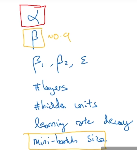
主要对于这几个超参数进行调试:
- $\alpha$ :学习率
- $\beta$ : momentum(0.9就是一个很好的值)
- $\beta1,\beta2,\epsilon$:
- layers:
-
**hidden units**
:
- learning rate decay:
-
**mini-batch size**
:保证算法运行有效
2.1随机取值and精确搜索
有粗糙到精细的进行参数的搜索,大概思想如下:
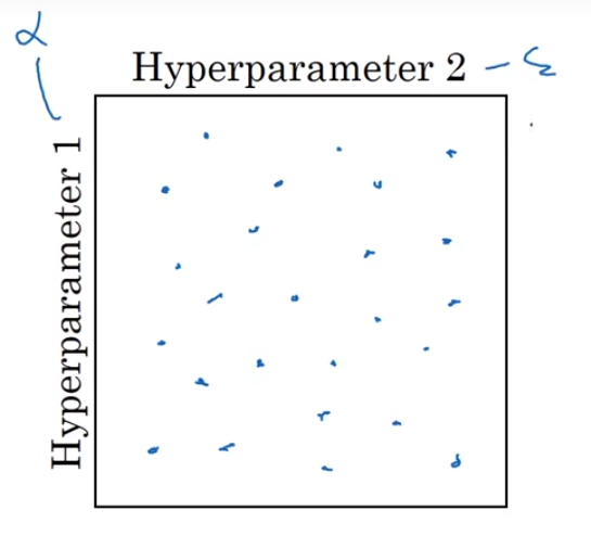
先对这一个范围内的数进行随机均匀取值(合适的步进值)来进行测试,找到效果最好的那个点。
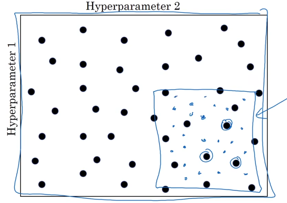
接着聚集于表现效果最好的参数点,对于其周围进行密集取值找到表现最好的点。
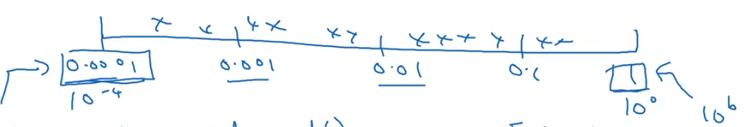
这里提到的均匀取值,可以考虑在对数坐标轴上分段进行随机均匀取值(减少计算量和资源占用)
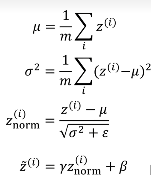
2.2Batch-Normalization
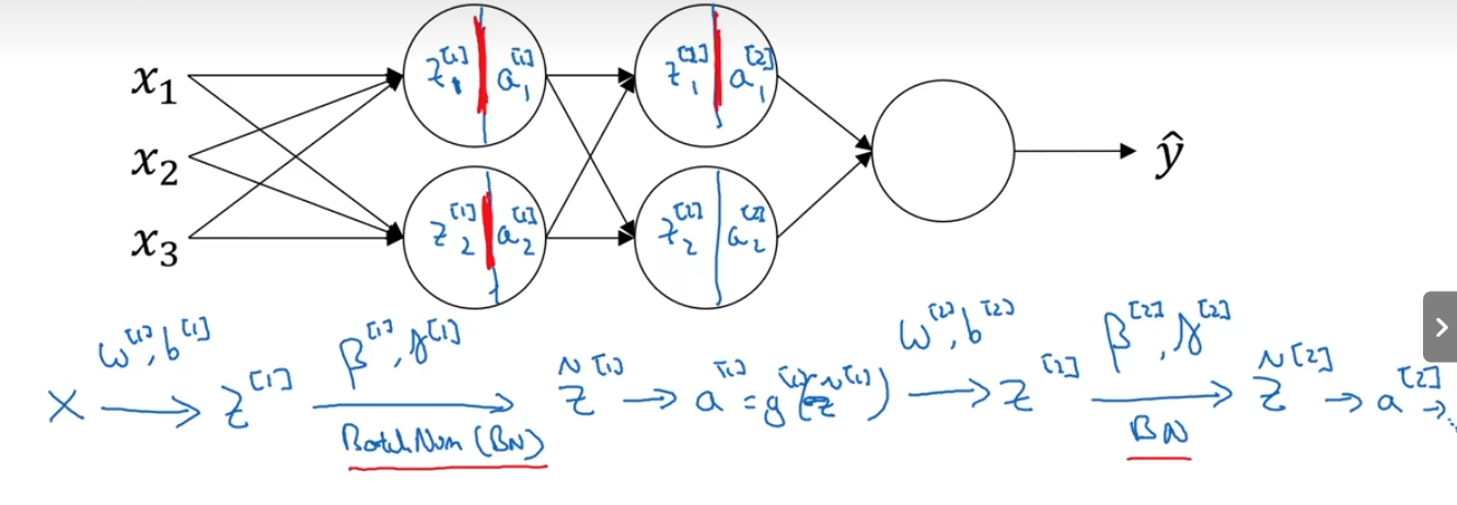
Batch-Normalization是发生在计算z和a之间。
Tensorflow中只需要一行代码:
tf.nn.batch-normalization()
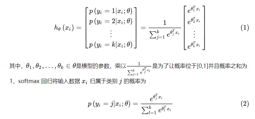
2.3Softmax回归
softmax 回归(softmax regression)其实是 logistic 回归的一般形式,logistic 回归用于二分类,而 softmax 回归用于多分类
对于输入数据{($x_1,y_1$),($x_2,y_2$),…,($x_m,y_m$)}有$k$个类别,即$y_i∈{1,2,…,k}$,那么 softmax 回归主要估算输入数据$x_i$ 归属于每一类的概率,即:
上面的式子可以用下图形象化的解析:
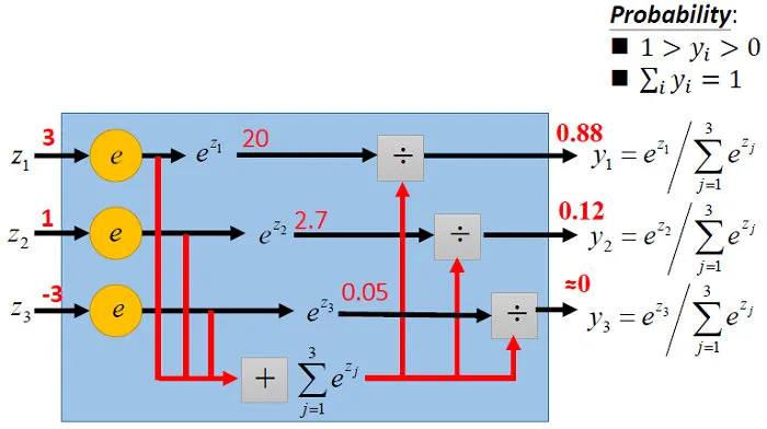
Softmax回归代码如下:
def load_dataset(file_path):
dataMat = []
labelMat = []
fr = open(file_path)
for line in fr.readlines():
lineArr = line.strip().split()
dataMat.append([1.0, float(lineArr[0]), float(lineArr[1])])
labelMat.append(int(lineArr[2]))
return dataMat, labelMat
def train(data_arr, label_arr, n_class, iters = 1000, alpha = 0.1, lam = 0.01):
'''
@description: softmax 训练函数
@param {type}
@return: theta 参数
'''
n_samples, n_features = data_arr.shape
n_classes = n_class
# 随机初始化权重矩阵
weights = np.random.rand(n_class, n_features)
# 定义损失结果
all_loss = list()
# 计算 one-hot 矩阵
y_one_hot = one_hot(label_arr, n_samples, n_classes)
for i in range(iters):
# 计算 m * k 的分数矩阵
scores = np.dot(data_arr, weights.T)
# 计算 softmax 的值
probs = softmax(scores)
# 计算损失函数值
loss = - (1.0 / n_samples) * np.sum(y_one_hot * np.log(probs))
all_loss.append(loss)
# 求解梯度
dw = -(1.0 / n_samples) * np.dot((y_one_hot - probs).T, data_arr) + lam * weights
dw[:,0] = dw[:,0] - lam * weights[:,0]
# 更新权重矩阵
weights = weights - alpha * dw
return weights, all_loss
def softmax(scores):
# 计算总和
sum_exp = np.sum(np.exp(scores), axis = 1,keepdims = True)
softmax = np.exp(scores) / sum_exp
return softmax
def one_hot(label_arr, n_samples, n_classes):
one_hot = np.zeros((n_samples, n_classes))
one_hot[np.arange(n_samples), label_arr.T] = 1
return one_hot
def predict(test_dataset, label_arr, weights):
scores = np.dot(test_dataset, weights.T)
probs = softmax(scores)
return np.argmax(probs, axis=1).reshape((-1,1))
if __name__ == "__main__":
#gen_dataset()
data_arr, label_arr = load_dataset('train_dataset.txt')
data_arr = np.array(data_arr)
label_arr = np.array(label_arr).reshape((-1,1))
weights, all_loss = train(data_arr, label_arr, n_class = 4)
# 计算预测的准确率
test_data_arr, test_label_arr = load_dataset('test_dataset.txt')
test_data_arr = np.array(test_data_arr)
test_label_arr = np.array(test_label_arr).reshape((-1,1))
n_test_samples = test_data_arr.shape[0]
y_predict = predict(test_data_arr, test_label_arr, weights)
accuray = np.sum(y_predict == test_label_arr) / n_test_samples
print(accuray)
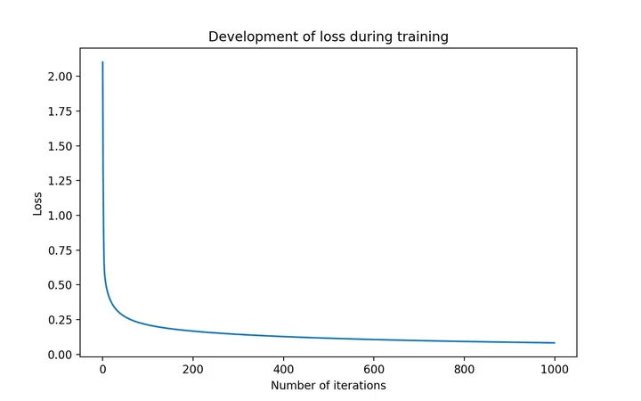
# 绘制损失函数
fig = plt.figure(figsize=(8,5))
plt.plot(np.arange(1000), all_loss)
plt.title("Development of loss during training")
plt.xlabel("Number of iterations")
plt.ylabel("Loss")
plt.show()
- 准确率:
0.9952
详细数据集和代码见此处:https://github.com/HuStanding/ml/tree/master/softmax