1.Lenet和现代经典卷积神经网络
手敲一遍过去三四十年的传统神经网络,加深一下对于网络演变的认识,给自己后续学习新进的网络结构打好基础。
主要是分为:
- 传统卷积神经网络:LeNet
- 现代卷积神经网络:AlexNet、VGG、NiN、GoogleLeNet、Resnet、DenseNet
2.传统卷积神经网络
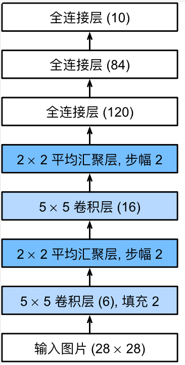
2.1LeNet

下面是简化版的LeNet
1 | import torch |
设置输入数据并输出每一层的形状,以此来检查模型
1 | X = torch.rand(size=(1,1,28,28),dtype=torch.float32) |
1 | Conv2d output shape: torch.Size([1, 6, 28, 28]) |
在整个卷积块中,与上一层相比,每一层特征的高度和宽度都减小了。第一个卷积层使用2个像素的填充,来补偿
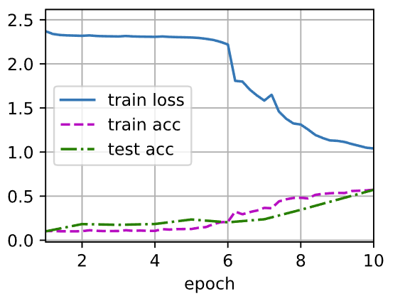
训练评估Lenet-5模型
1 | batch_size = 256 |
总结:
- 为了构造高性能的卷积神经网络,我们通常对卷积层进行排列,逐渐降低其表示的空间分辨率,同时增加通道数。
- 在传统的卷积神经网络中,卷积块编码得到的表征在输出之前需由一个或多个全连接层进行处理。
3.现代经典卷积神经网络
3.1AlexNet
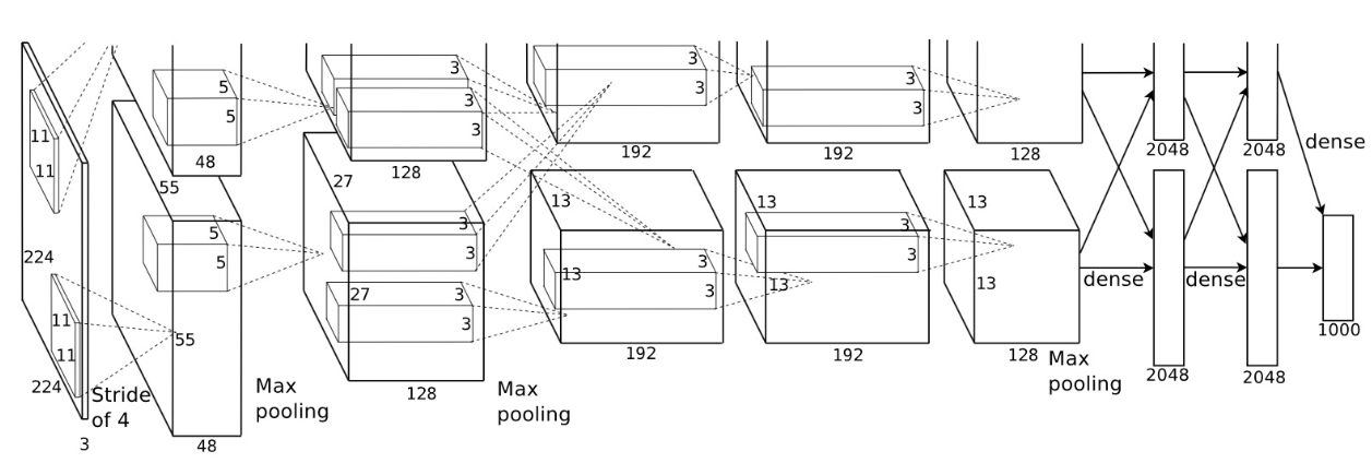
模型设计:
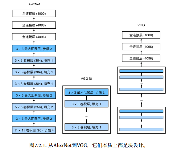
因为ImageNet大多数图像的宽高比MINIST多十倍,因此需要更大的卷积窗口来捕获特征,所以第一层卷积窗口形状是11X11。第二层中的卷积窗口形状被缩减为5 × 5,然后是3 × 3。此 外,在第一层、第二层和第五层卷积层之后,加入窗口形状为3 × 3、步幅为2的最大汇聚层。而且,AlexNet的 卷积通道数目是LeNet的10倍。
和LeNet还有一点不同的是,AlexNet使用RELU激活函数替换掉了原来的Sigmoid激活函数。
1 | import torch |
1 | X = torch.randn(1,1,224,224) |
输出网络形状变化:
1 | Conv2d output shape torch.Size([1, 96, 54, 54]) |
训练:
1 | batch_size = 128 |
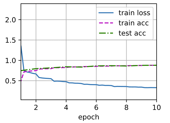
输出:
3.2VGG
本质上是块的累积,更大更深的AlexNet
说明:
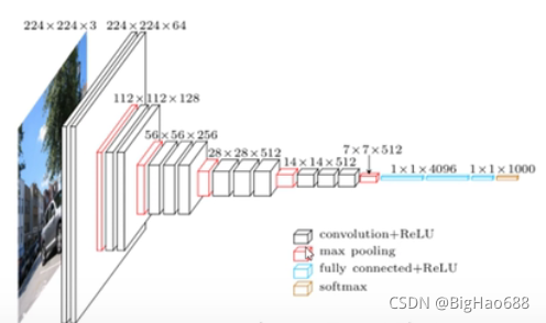
白色矩形框:代表卷积和激活函数
红色矩形框:代表最大池化下载量
蓝色矩形框:全连接层和激活函数
橙色矩形框:softmax处理
结构过程:(配置表和结构图一起观察)
1、首先输入一张2242243大小的图像,经过两个33的卷积层之后,所得到的特征图大小为224224*64(尺寸大小不变,因为采用的是64个卷积核,所以深度也为64)。
2、通过一个最大池化下载量层,得到的特征图为11211264(大小缩小一半,不改变深度)。
3、再通过两个33128的卷积层,得到的特征图为112112128(深度变为128)。
4、通过一个最大池化下载量层,得到的特征图为5656128(大小缩小一半,不改变深度)。
5、再通过三个33256的卷积层,得到的特征图为5656256(深度变为256)。
6、通过一个最大池化下载量层,得到的特征图为2828256(大小缩小一半,不改变深度)。
7、再通过三个33512的卷积层,得到的特征图为2828512(深度变为512)。
8、通过一个最大池化下载量层,得到的特征图为1414512(大小缩小一半,不改变深度)。
9、再通过三个33512的卷积层,得到的特征图为1414512(深度变为512)。
10、通过一个最大池化下载量层,得到的特征图为77512(大小缩小一半,不改变深度)。
11、再通过两个为4000个节点的全连接层以及激活函数,得到114096向量
12、再通过一个为1000个节点的全连接层(因为1000个类别),注意不需要激活函数,得到111000向量。
13、最后将通过全连接层得到的一维向量,输入到softmax激活函数,将预测结果转化为概率分布。
模型设计:
1 | import torch |
模型形状输出:
1 | Sequential output shape torch.Size([1, 64, 112, 112]) |
训练模型:
1 | #训练模型 |
3.3NiN
1 | import torch |
总结:
- NiN使用由一个卷积层和多个
卷积层组成的块。该块可以在卷积神经网络中使用,以允许更多的每像素非线性。 - NiN去除了容易造成过拟合的全连接层,将它们替换为全局平均汇聚层(即在所有位置上进行求和)。该汇聚层通道数量为所需的输出数量(例如,Fashion-MNIST的输出为10)。
- 移除全连接层可减少过拟合,同时显著减少NiN的参数。
- NiN的设计影响了许多后续卷积神经网络的设计。
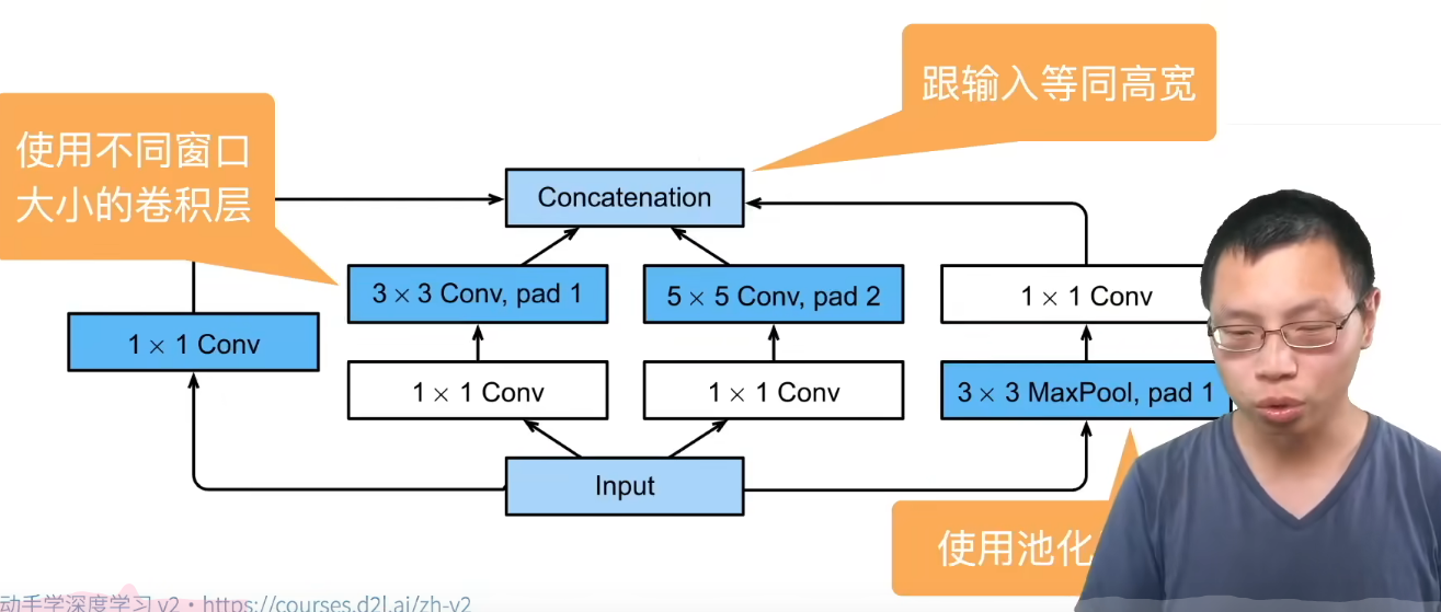
3.4GoogLeNet
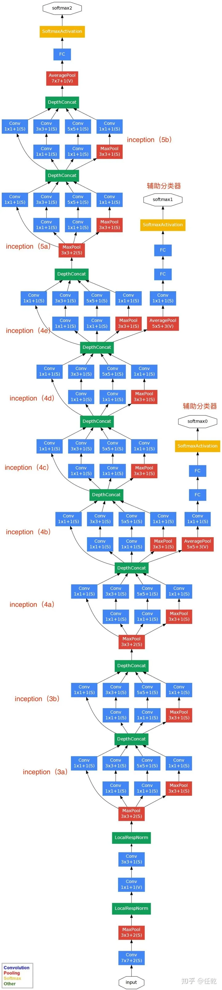
核心:提出了Inception块,它是把多个卷积或池化操作,放在一起组装成一个网络模块,设计神经网络时以模块为单位去组装整个网络结构。
模型实现:
- 首先实现关键的Inception模块:
1 | import torch |
- 利用Inception实现GoogLeNet模块:
1 | # 实现GoogleNet的各个模块 |
- 创建样例数据并输出模型形状结构:
1 | #创建样例数据 |
输出:
1 | Sequential output shape: torch.Size([1, 64, 26, 26]) |
- 训练:
1 | lr,num_epochs,batch_size = 0.1,10,128 |
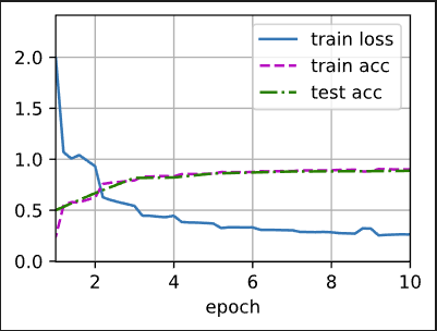
训练结果:
3.5BatchNorm(补充知识)
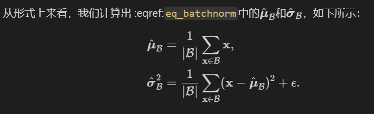
本质上就是将通道层作为卷积层,利用小批量的均值和标准差,不断调整神经网络的中间输出,使整个神经网络各层的中间输出值更加稳定。
从形式上来说,用
对于全连接层处批量归一化计算通常,我们将批量规范化层置于全连接层中的仿射变换和激活函数之间。
设全连接层的输入为x,权重参数和偏置参数分别为
那么,使用批量规范化的全连接层的输出的计算详情如下:
均值和方差是在应用变换的"相同"小批量上计算的。
构建并测试:
- 构建一个具有张量的批量规划化层:
1 | import torch |
- 集成到自定义层中(处理数据移动到GPU上、分配初始化任何必须的变量、跟踪移动平均线“均值、方差”)
1 | class BatchNorm(nn.Module): |
- 部署BatchNorm到LeNet中:
1 | net = nn.Sequential( |
- 输出:
1 | loss 0.271, train acc 0.899, test acc 0.821 |
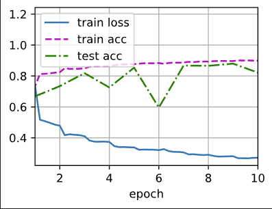
3.6ResNet
越来越深越复杂的网络并不代表性能越来越好,达到一个阈值之后就会出现一个瓶颈(前面层数提取到的特征很大一部分会丢失)。
而ResNet层利用一个残差块加入快速通道来尽可能保留前面卷积层保留的参数。输入可通过跨层数据线路更快地向前传播。
模型构建:
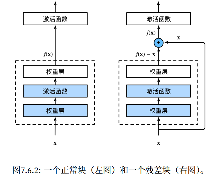
- 残差块模块:
1 | import torch |
- ResNet整体模型构建:
1 | #构建ResNet整体模型 |
模型形状变化:
1 | Sequential output shape/t torch.Size([1, 64, 56, 56]) |
- 训练模型:
1 | #训练模型 |
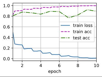
输出:
1 | loss 0.012, train acc 0.997, test acc 0.893 |
小结:
- 学习嵌套函数(nested function)是训练神经网络的理想情况。在深层神经网络中,学习另一层作为恒等映射(identity function)较容易(尽管这是一个极端情况)。
- 残差映射可以更容易地学习同一函数,例如将权重层中的参数近似为零。
- 利用残差块(residual blocks)可以训练出一个有效的深层神经网络:输入可以通过层间的残余连接更快地向前传播。
- 残差网络(ResNet)对随后的深层神经网络设计产生了深远影响。
3.7DenseNet
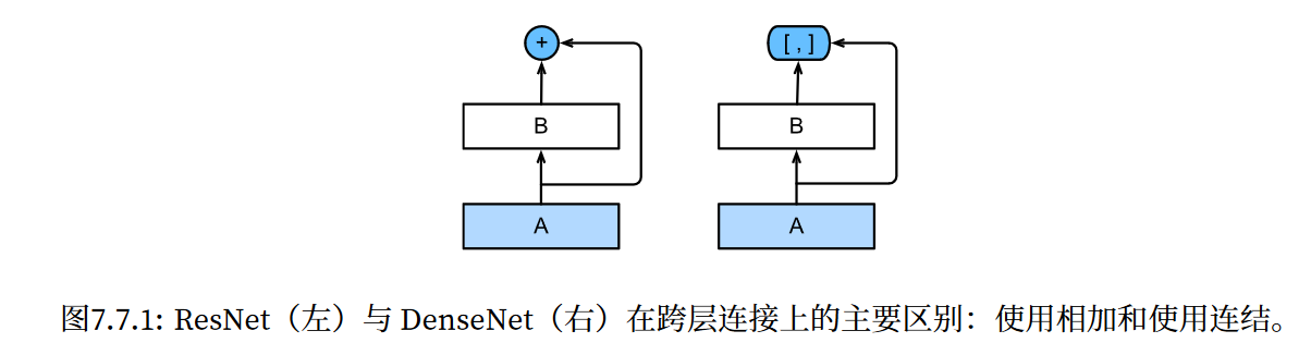
ResNet和DenseNet的关键区别在于,DenseNet输出是连接(用图中的[, ]表示)而不是 如ResNet的简单相加。因此,在应用越来越复杂的函数序列后,我们执行从x到其展开式的映射:

最后,将这些展开式结合到多层感知机中,再次减少特征的数量。
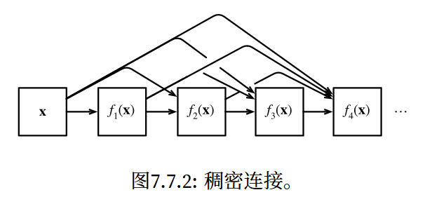
稠密网络主要由2部分构成:稠密块(dense block)和过渡层(transition layer)。前者定义如何连接输入和 输出,而后者则控制通道数量,使其不会太复杂。
构建模型:
1 | import torch |
接着我们开始构建DenseNet,DenseNet首先使用同ResNet一样的单卷积层和最大汇聚层。
1 | b1 = nn.Sequential( |
接下来,类似于ResNet使用的4个残差块,DenseNet使用的是4个稠密块。与ResNet类似,我们可以设置每个稠密块使用多少个卷积层。这里我们设成4,从而与
sec_resnet的ResNet-18保持一致。稠密块里的卷积层通道数(即增长率)设为32,所以每个稠密块将增加128个通道。在每个模块之间,ResNet通过步幅为2的残差块减小高和宽,DenseNet则使用过渡层来减半高和宽,并减半通道数。
1 | # num_channels为当前的通道数 |
利用如下代码来观察DenseNet网络每层的形状:
1 | X = torch.rand(size=(1,1,224,224)) |
输出:
1 | Sequential output shape torch.Size([1, 64, 56, 56]) |
训练:
1 | lr, num_epochs, batch_size = 0.1, 10, 256 |
1 | loss 0.140, train acc 0.948, test acc 0.885 |

小结:
- 在跨层连接上,不同于ResNet中将输入与输出相加,稠密连接网络(DenseNet)在通道维上连结输入与输出。
- DenseNet的主要构建模块是稠密块和过渡层。
- 在构建DenseNet时,我们需要通过添加过渡层来控制网络的维数,从而再次减少通道的数量。
4.总结
上述复现了过去几十年卷积神经网络的经典网络并进行测试训练,同时也学习了BatchNorm(不能提高准确率,只能够提高收敛速度)。